


Question 1 - How to create a Table
How to Create a Table in Excel 2010
By Greg Harvey from Excel 2010 For Dummies
1 of 12 in Series: The Essentials of Working with Tables in Excel 2010
You can create a table in Excel 2010 to help you manage and analyze related data. The purpose of an Excel table is not so much to calculate new values but rather to store lots of information in a consistent manner, making it easier to format, sort, and filter worksheet data.
1
Enter your table's column headings.
Click the blank cell where you want to start the new table and then enter the column headings (such as ID No, First Name, Last Name, Dept, and so on) in separate cells within the same row. Column headings are also known asfield names. The column headings should appear in a single row without any blank cells between the entries.
2
Enter the first row of data immediately below the column headings you typed in Step 1.
These entries constitute the first row, or record, of the table.

4
Click the My Table Has Headers check box to select it.
These headers are the column headings entered in the first step.

5
Click OK.
Excel inserts and formats the new table and adds filter arrows (drop-down buttons) to each of the field names in the top row.
Another way to insert a table is to click the Format as Table button in the Styles group on the Home tab and then select a table style of your choice in the gallery that appears. Use this method if you want to apply a different table style as you create a table.
If you want to convert an existing Excel table back to a normal range of cells, select any cell in the table and then click the Convert to Range button on the Table Tools Design tab. All data and formatting is preserved.
Answer
Formulas are what helped make spreadsheets so popular. By creating formulas, you can have instantaneous calculations whenever changing any information in cells the formula is looking at.
The basics
All spreadsheet formulas begin with =
After the equal symbol either the cell or formula function is entered. The function tells the spreadsheet what kind of formula it's dealing with.
If a function is being performed the math formula or cells being dealt with are surrounded in parentheses.
Using the colon (:) will allow you to get a range of cells for a formula.
Formula examples
Note: The functions listed below may not be the same in all languages of Microsoft Excel. All these examples are done in the English version of Microsoft Excel.
=
= will create a cell equal to another. For example, if you were to put =A1 in B1 what ever was in A1 would automatically be put in B1. You could also create a formula that would make one cell equal to more than one value. For example, if you have a first name in cell A1 and a last name in cell B1, you could put in cell A2 =A1&" "&B1 which would put cell A1 in with B1 with a space between.
=AVERAGE(X:X)
Display the average amount between cells. For example, if you wanted to get the average for cells A1 to A30, you would type: =AVERAGE(A1:A30)
=COUNTIF(X:X,"*")
Count the cells that have a certain value. For example, if you had =COUNTIF(A1:A10,"TEST") put in cell A11 then anywhere between A1 through A10 that has the word test would be counted as 1, so if you had 5 cells that had the word test A11 would say 5.
=IF(*)
The syntax of the IF statement are =IF(CELL="VALUE" ,"PRINT OR DO THIS","ELSE PRINT OR DO THIS"). So a good example of the syntax would be =IF(A1="","BLANK","NOT BLANK"), this would make any cell besides cell A1 say "BLANK" if a1 had nothing within it, and "NOT BLANK" if any information was within it. The if statement can, of course, become a lot more complicated but can be reduced if following the above structure.
=MEDIAN(A1:A7)
Find the median of the values of cells A1 through A7. For example, four is the median for 1, 2, 3, 4, 5, 6, 7.
=MIN/MAX(X:X)
Min and Max represent the minimum or maximum amount in the cells. For example, if you wanted to get the minimum value between cells A1 and A30 you would put =MIN(A1:A30) or if you wanted to get the Maximum about =MAX(A1:A30).
=Product(X:X)
Multiples multiple cells together. For example =Product(A1:A30) would multiple all cells together, so A1 * A2 * A3, etc.
=SUM(X:X)
The most commonly used function to add, subtract, multiple, or divide values in cells. Below are some examples.
=SUM(A1+A2)
Add the cells A1 and A2.
=SUM(A1:A5)
Add cells A1 through A5.
=SUM(A1,A2,A5)
Adds cells A1, A2, and A5.
=SUM(A2-A1)
Subtract cell A2 from A1.
=SUM(A1*A2)
Multiply cells A1 and A2.
=SUM(A1/A2)
Divide cells A1 and A2.
=SUMIF(X:X,"*"X:X)
Perform the SUM function only if there is a specified value in the first selected cells. An example of this would be =SUMIF(A1:A6,"TEST",B1:B6) which only adds the values B1:B6 if the word "test" was put somewhere in between A1:A6. So if you put TEST (not case sensitive) in A1, but had numbers in B1 through B6, it would only add the value in B1 because TEST is in A1.
=TODAY()
Would print out the current date in the cell entered. This value will change to reflect the current date each time you open your spreadsheet. If you want to enter a date that doesn't change hold down CTRL and ; to enter the date.
=TREND(X:X)
To find the common value of cell. For example, if cells A1 through A6 had 2,4,6,8,10,12 and you entered formula =TREND(A1:A6) in a different cell, you would get the value of 2 because each number is going up by 2.
=VLOOKUP(X,X:X,X,X)
The lookup, hlookup, or vlookup formula allows you to search and find related values for returned results. See our lookup definition for a complete definition and full details on this formula.
3. How to insert Symbol RM with 2 decimal places.
How to Insert Decimal Points Automatically in Excel 2010
By Greg Harvey from Excel 2010 For Dummies
If you need to enter a bunch of numbers in an Excel 2010 worksheet that use the same number of decimal places, you can turn on Excel’s Fixed Decimal setting and have the program enter the decimals for you. All you do is type the digits and complete the entry in the cell.
For example, to enter the numeric value 100.99 in a cell after fixing the decimal point to two places, type the digits 10099 without typing the period for a decimal point. When you complete the cell entry, Excel automatically inserts a decimal point two places from the right in the number you typed, leaving 100.99 in the cell.
To fix the number of decimal places in a numeric entry, follow these steps:
2
Click the Advanced tab.
The Advanced options appear in the right pane.
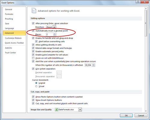
3
Select the Automatically Insert a Decimal Point check box in the Editing Options section.
By default, Excel fixes the decimal place two places to the left of the last number you type. To change the default Places setting, go to Step 4; otherwise move to Step 5.
4
(Optional) Type a new number in the Places text box or use the spinner buttons to change the value.
For example, you could change the Places setting to 3 to enter numbers with the following decimal placement: 00.000.

5
Click OK.
If you want to enter a number without a decimal point while the Fixed Decimal setting is turned on, or one with a decimal point in a position different from the one called for by this feature, you have to type the decimal point yourself. For example, to enter the number 1099 instead of 10.99 when the decimal point is fixed at two places, type 1099 followed immediately by a period (.) in the cell.
When you’re ready to return to normal data entry for numerical values (where you enter any decimal points yourself), open the Advanced tab of the Excel Options dialog box and then select the Automatically Insert a Decimal Point check box again, this time to clear it, and click OK.
Conclusion ;
I have learn how to create the table , learn to made mathematic formula , and i have learn to insert symbol RM with two decimal places.
No comments:
Post a Comment